Lecture notes
From a course by Anne M. Ruiz and Colombe Becquart.

1 Generalities
1.1 Data
Typical applications of discriminant analysis include credit scoring, quality control, and risk prediction.
We assume that the data consist of \(n\) observations described by \(p\) quantitative variables. The observations belong to \(k < p\) classes or groups, which are represented by a qualitative variable with \(k\) categories. The data are stored in a table with \(n\) rows (observations) and \(p+1\) columns (variables, including the qualitative variable).
Let \(X^1, X^2, \ldots, X^p\) denote the \(p\) quantitative variables, which will be considered as explanatory variables. Let \(Y\) denote the qualitative variable, which is the variable to be explained.
1.2 Objectives
The primary objective of discriminant analysis (DA) is to separate the \(k\) classes as effectively as possible using the \(p\) explanatory variables. To achieve this, DA constructs new variables called discriminant variables. These variables can then be used to produce graphical representations that illustrate the separation of the \(k\) groups based on the \(p\) explanatory variables.
The second objective of DA is to classify a new observation, described by these \(p\) quantitative variables, into one of the \(k\) groups (also called group allocation).
Remark 1. As in regression, DA is formulated as an explanatory model. The main difference is that the variable to be explained is qualitative rather than quantitative.
1.3 Linear discriminant variables (heuristics)
A linear discriminant variable is a linear combination of the \(p\) explanatory variables that separates the \(k\) groups as effectively as possible.
In general, at most \(k-1\) discriminant functions are sufficient to separate \(k\) classes.
Remark 2. Discriminant analysis is conceptually similar to principal component analysis (PCA) in that we search for new variables that are linear combinations of the original variables. However, whereas PCA aims to preserve total variance (inertia), DA aims to maximize the separation between groups or classes.
2 Discriminant Analysis
2.1 Between-group and within-group variances
Instead of computing the mean vector and covariance matrix for the entire dataset, DA computes them separately for each class.
Let \(n_1, n_2, \ldots, n_k\) denote the number of observations in each class. Let \[ \overline{X^1}^{(1)}, \overline{X^1}^{(2)}, \ldots, \overline{X^1}^{(k)} \] denote the mean of variable \(X^1\) within each class, and similarly for \(X^2, \ldots, X^p\). Let \[ \overline{X}^{(1)}, \overline{X}^{(2)}, \ldots, \overline{X}^{(k)} \] denote the mean vectors for each class.
In the same manner, we compute the covariance matrices for each class, denoted \(V^{(j)}, j=1,\ldots,k\).
The total covariance matrix for all observations is: \[ V = \frac{1}{n} \sum_{i=1}^n (X_i - \overline{X})(X_i - \overline{X})^\top. \]
We define two important matrices: the within-group and between-group covariance matrices.
In discriminant analysis, we seek discriminant variables that maximize the between-group variance while minimizing the within-group variance. This contrasts with PCA, which maximizes total variance without considering group structure.
Remark 3. In regression terms, TSS (total sum of squares) corresponds to \(V\), ESS (explained sum of squares) corresponds to \(B\), and RSS (residual sum of squares) corresponds to \(W\).
2.2 Mahalanobis Distance
For two vectors \(u\) and \(v\) in \(\mathbb{R}^p\), the Euclidean distance is \[ d^2(u,v) = \sum_{i=1}^p (u_i - v_i)^2 = (u-v)^\top (u-v). \]
2.3 Steps of the analysis
2.3.1 Computing discriminant variables
We start by computing the eigendecomposition of: \[ W^{-1} B \] (instead of the correlation matrix \(R\) in PCA).
2.3.2 Global quality of discrimination
The squared canonical correlation coefficient: \[ \frac{\operatorname{Var}_B(\operatorname{CAN}^j)}{\operatorname{Var}(\operatorname{CAN}^j)} =\frac{\lambda_j}{1+\lambda_j} \] (where \(\lambda_j\) is the eigenvalue associated with the \(j\)-th discriminant variable) measures the proportion of variance of a discriminant variable explained by the between-group variance, analogous to \(R^2\) in regression. Values close to 1 indicate strong discrimination.
2.3.3 Dimension choice
When more than two discriminant variables exist, a choice of which to retain is required. The importance of a discriminant variable decreases with its order, and explained inertia can be used as a criterion, measured by the eigenvalues.
2.3.4 Interpretation of the discriminant variables
Coefficients (raw canonical coefficients) indicate the contribution of each variable. Correlations between the initial variables and discriminant variables can also be visualized using scatterplots.
2.3.5 Scatterplot of the observations on the discriminant axes
We plot the discriminant variables (CAN1, CAN2, . . . ) which correspond to the coordinates of the observations on these new variable and use different symbols or colors to visualize the different categories of the variable we explain.
If we have many discriminant variables, we can plot different scatterplots: (CAN1,CAN2), (CAN1,CAN3),… (similar to PCA).
Remark: In the presence of 2 groups, only one discriminant variable. Plot an histogram in that case with different colors depending on the value of the categorical variable.
2.3.6 Interpretation
All the observations can be interpreted (there is no problem of quality of representation). We interpret the scatterplot in terms of discrimination of the groups (which axis discriminate which group? How good is the discrimination?) We also make comment on the groups which are not well separated.
Remark. In some cases, the discrimination is not perfect with some overlapping of some the groups on the scatterplots and this also deserves comment.
3 Allocation (or classification) rule
We now consider the second objective of discriminant analysis. Once the discriminant variables obtained (which lead to the best separation between groups), some new observation is considered for which we only know the explanatory variables and do not know the explained variable (category of the qualitative variable or group). Our aim is to allocate this new observation to one of the \(k\) groups (prediction objective).
There exist several possibilities to allocate or classify an observation to one of the \(k\) possible groups. We will give details on an intuitive (geometric) allocation rule but there exist many more based on probabilistic arguments and we will present briefly one of them.
3.1 Geometric classification rule
The idea is simple and consists of calculating for a given observation its discriminant variables and allocating the observation to the group with the nearest mean. Because the distances are calculating on the discriminant variables (using the usual Euclidean formula), it takes into account the Mahalanobis distance. In order to implement this allocation rule, we need to know the mean of each class and the values of the observations all for the discriminant variables:
\[f(x) = \arg\min_{1 \leq g \leq k} d_W^2 (x, \overline{X}^{(g)})\]
Example 1 If the group means are symmetric around 0, a positive CAN1 value indicates assignment to group 1, and a negative value indicates assignment to group 2.
Remark 4. The geometric classification rule leads to the prediction of a group for a new observation. This rule may lead to some errors if the groups are not well separated. The major problem with the geometric rule is that it does not take into account the possibility of unbalanced groups (for some rare events for instance). The following rule will correct this problem.
3.2 Probabilistic classification rules
If we assume a Gaussian distribution within each group, and known prior probabilities, we can compute the posterior probabilities for each observation and assign it to the group with the highest posterior probability (Bayes rule). When we assume that all the within-group covariance matrices are equal to \(W\), then we obtain the rule: \[f(x) = \arg\min_{1 \leq g \leq k} d_W^2 (x, \overline{X}^{(g)}) - 2 \log \frac{n_g}n\]
3.3 Quality of classification
3.3.1 Confusion matrix
In order to measure the quality of classification rules, one applies the rules to observations for which we already know the group and compare the predictions with the actual values in a confusion table.
If the categorical variable has \(k\) categories and we classify \(n\) observations, the confusion matrix contains \(k\) columns which correspond to the \(k\) actual categories and \(k\) rows for the \(k\) predicted categories. Each of the \(n\) observations is assigned to the corresponding cell of the table which contains the cross-tabulated counts.
| actual class 1 | actual class 2 | … | actual class k | |
|---|---|---|---|---|
| predicted class 1 | \(n_{11}\) | \(n_{12}\) | … | \(n_{1k}\) |
| predicted class 2 | \(n_{21}\) | \(n_{22}\) | … | \(n_{2k}\) |
| … | ||||
| predicted class k | \(n_{k1}\) | \(n_{k2}\) | … | \(n_{kk}\) |
The sum of all \(n_{ij}\) is \(n\).
In the case of only two-classes, we have:
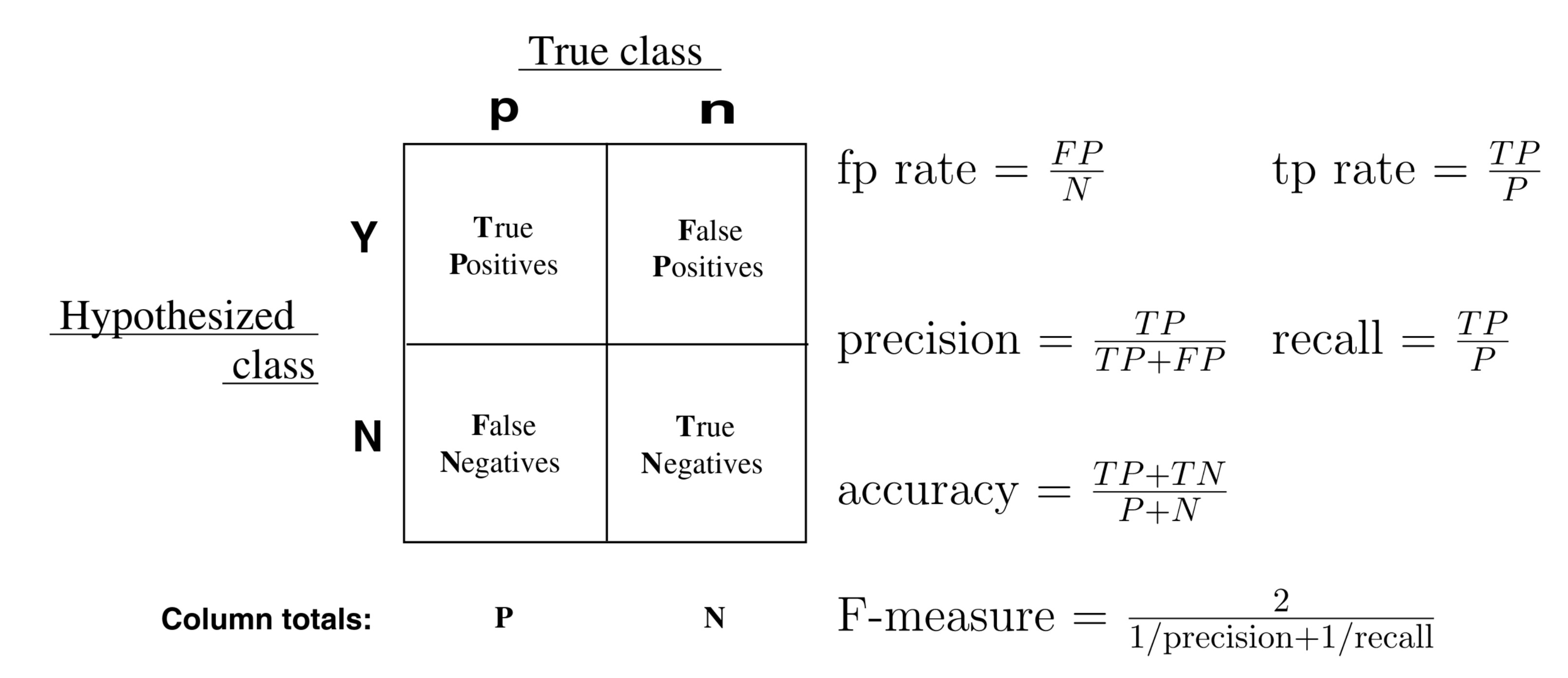
Remark 5. Sensitivity = True Positive Rate (TPR) = Hit = Recall.
Specificity = 1 - False Positive Rate (FPR).
3.3.2 ROC and AUC
In the case where \(k=2\), we can represent the classification rule of LDA as a ROC (receiver operating characteristic) curve. Each classification rule is represented as a point in the ROC space, which is the \([0,1]^2\) square where the x-axis is the FPR and the y-axis is the TPR.
The diagonal correspond to flip-a-coin classification, whereas the left and upper boundaries of the square correspond to perfect classification.
Since LDA produces scores (posterior probabilities) rather than binary class labels, we can choose a threshold to convert scores into class assignments. By varying this threshold from the extreme that assigns all observations to class 1 to the extreme that assigns all to class 2, we obtain a ROC curve, representing all possible classification rules associated with the considered discriminant analysis.
Then, the AUC (area under the curve) provides a global measurement of the performance of LDA as a classification method.
4 Invariant Coordinate Selection (ICS)
If the group are unknown a priori, the between-group and within-group covariance matrices are not computable, so it is impossible to perform a discriminant analysis.
But Invariant Coordinate Selection can recover the discriminant subspace without knowing the groups by replacing the between-group and within-group covariance matrices by two scatter matrices.
4.1 General principle
The objective of Invariant Coordinate Selection is to maximize the ratio of two scatter matrices capturing the ratio of \(B\) to \(W\) : \[\max_{\substack{v \in \mathbb{R}^p}} \frac{v^\top\operatorname{Cov}_4[X]v}{v^\top\operatorname{Cov}[X]v}\]
4.2 Scatter matrices
Let \(X\) be a random vector of dimension \(p\), with distribution function \(F_X\). A scatter matrix of \(X\), denoted \(V(F_X)\), is a symmetric positive definite matrix of dimension \(p \times p\) and affine equivariant. Let \(\mathcal{P}_p\) be the set of all positive definite symmetric matrices of order \(p\).
\[\operatorname{Cov}[X]=\mathbb{E}[(X - \mathbb{E}(X))(X - \mathbb{E}(X))^\top]\]
\[\operatorname{Cov}_4[X]=\frac{1}{p+2} \mathbb{E}[d^2(X - \mathbb{E}(X))(X - \mathbb{E}(X))^\top]\] where \(d^2\) is the square of the Mahalanobis distance: \[d^2={(X - \mathbb{E}(X))^\top\operatorname{Cov}[X]^{-1}(X - \mathbb{E}(X))}\]
4.3 Component calculations
To perform this comparison, ICS relies on the joint diagonalization of \(V_1\) and \(V_2\). \[\begin{aligned} H^\top V_1H &= I_p \\ H^\top V_2H &= \Delta \end{aligned}\] where \(V_1, V_2 \in \mathcal{P}_p\), \(\Delta = \text{diag}(\rho_1, \dots, \rho_p)\), \(\rho_1, \dots, \rho_p\) being the eigenvalues of \(V_1^{-1}V_2\) sorted in descending order, and \(H = (h_1, \dots, h_p)\) is a matrix containing the corresponding eigenvectors.
The components are : \(Z = H^\top(Y - \mathbb{E}(Y))\)
4.4 Discriminant subspace
Let \(Y\) be a random vector following a mixture of \(k\) Gaussian distributions with the same covariance matrix : \[Y \sim \sum_{j=1}^{k}\alpha_j N_p(\mu_j, \Gamma)\] where \(\alpha_j > 0\) for \(j=1,\dots, k\) and \(\sum_{j=1}^{k}\alpha_j = 1\), \(\mu_j \in \mathbb{R}^p\) for \(j=1,\dots, k\), and \(\Gamma \in \mathcal{P}_p\).
The discriminant subspace \(\phi\) is given by : \[\phi = \langle \phi_1, \ldots, \phi_k \rangle\] where \(\phi_j = \Gamma^{-1} (\mu_j - \mu)\) for \(j=1,\ldots, k\).
4.5 Properties
The first and last invariant components generate the Fisher discriminant subspace, under certain conditions.
A certain number of eigenvalues will be equal, while the remainder will be either larger or smaller than the equal ones.
The first (last) components are associated with the largest (smallest) eigenvalues.
Thus, the focus of our analysis will be on the largest and/or smallest eigenvalues.
The components associated with non-equal eigenvalues are invariant under affine transformations, up to a factor of \(\pm 1\).
5 Conclusion
Discriminant analysis is appropriate when:
- Observations are described by quantitative variables and belong to distinct groups.
- The goal is to separate these groups using quantitative variables.
- We wish to classify new observations into one of the groups.
- The number of groups \(k\) is smaller than the number of variables \(p\).
Remark 6. This lecture covers linear discriminant analysis (canonical). Quadratic discriminant analysis is an extension that allows for group-specific covariance matrices.