Complex data structures
In this course, we will often assume that each of the \(n\) observations can be represented as a vector
\[
X_i \in \mathbb{R}^p.
\] In other words, a fixed number of numerical variables is measured for each individual.
However, many modern datasets do not fit into this framework. Instead of vectors, observations may be:
- functions
- probability distributions
- networks or graphs
- combinations of heterogeneous objects.
Such data are referred to as complex data.
Most classical methods covered in this course (PCA, LDA, CART, Random Forests) assume that we observe independent discrete random vectors in a Euclidean space.
Complex data invalidate this assumption. We need to understand their structure before applying any statistical or machine learning method.
This leads to new representations, metrics and notions of variability that are beyond the scope of this course.
Functional Data
In functional data analysis (FDA), each observation is a function: \[
f_i(t), \quad t \in \mathcal{T},
\] where \(\mathcal{T}\) is typically time, space, or wavelength.
Examples:
- daily electricity consumption curves,
- intraday financial price curves,
- yield curves in economics,
- temperature curves over a year.
Each observation is not a vector, but an entire curve.
Key challenges:
- Infinite-dimensional nature of the data
- Smoothness and regularity assumptions
- Temporal dependence within each observation.
Typical tools:
- Functional PCA
- Basis expansions (Fourier, splines, wavelets)
- Functional regression
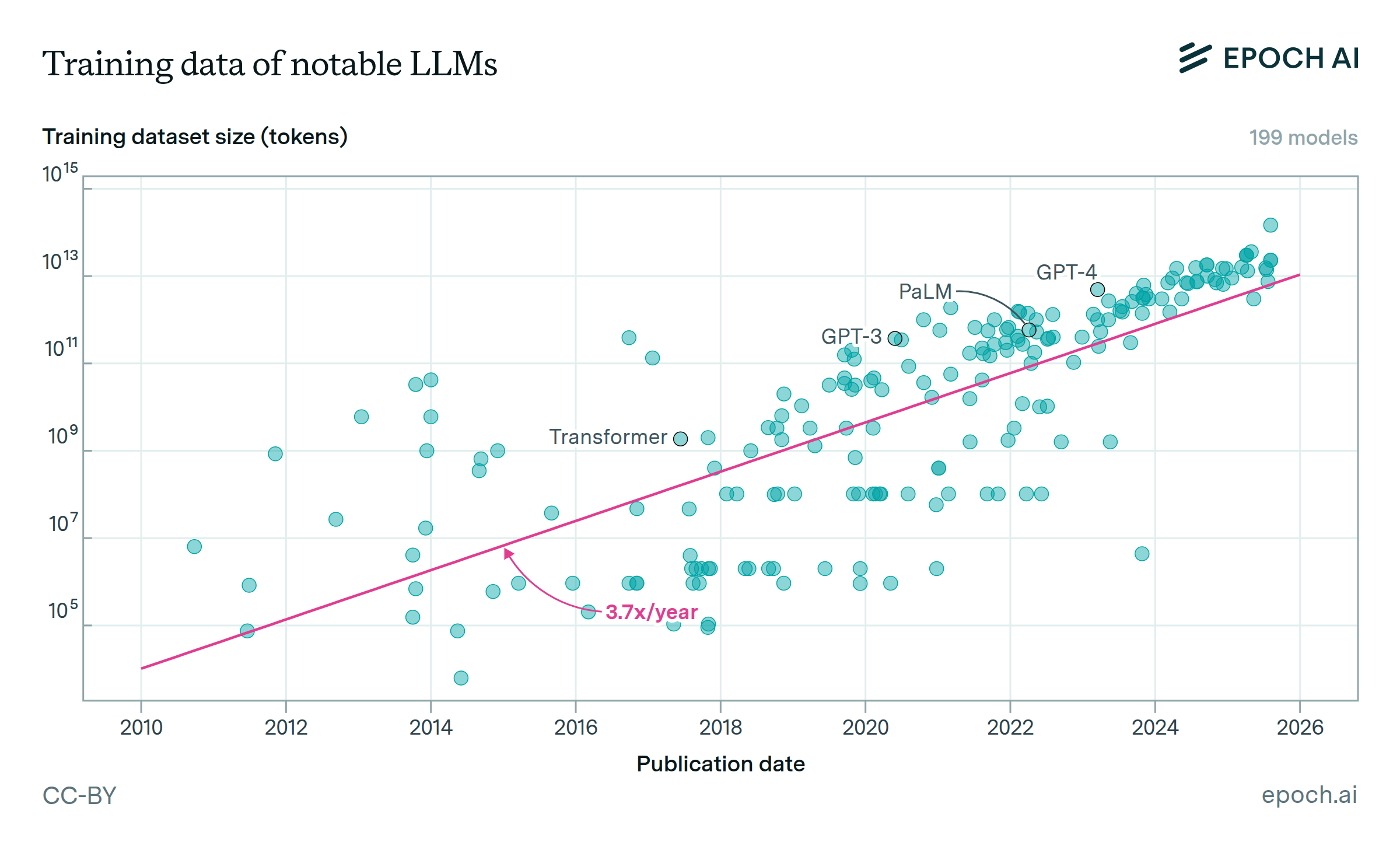
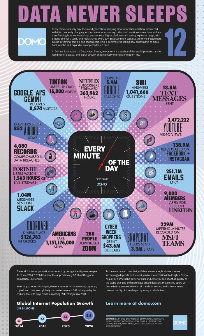
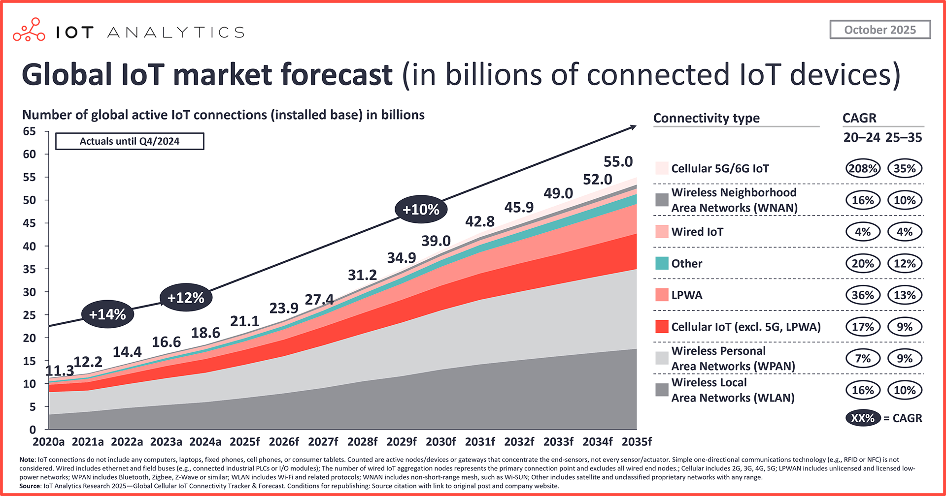
Functional data emerged as a consequence of the rising number of IoT devices monitoring variables at a very high frequency, that are better analyzed as continuous curves rather than discrete numerical values.
Distributional Data
In distributional data analysis (DDA), each observation is a probability distribution: \[
\pi_i (x), \quad x \in \mathcal X
\] (taking positive values and integrating to 1) rather than a single realization.
Examples:
- income distributions across regions,
- age distributions in populations,
- uncertainty-aware measurements,
- empirical distributions of prices or returns.
- temperature distributions over a year.
Key challenges:
- Standard distances (Euclidean) are meaningless
- How to average distributions?
Typical tools:
- Wasserstein (optimal transport) distances
- Fréchet means of distributions
- Aitchison structure (similar to compositional data).
Graph and Network Data
In graph data, each observation is a network: \[
G_i = (V_i, E_i),
\] with nodes \(V_i\) and edges \(E_i\).
Examples: social networks, trade networks.
Key challenges: Size and topology vary across graphs. Dependence structure is intrinsic. Graphs encode relational information, not just attributes.
Typical tools:
- Graph Laplacians and spectral methods
- Network embeddings
- Graph neural networks.
Other kinds of complex data
- Textual Data
- Documents, articles, social media posts
- Represented via embeddings or topic models
- High-dimensional, sparse, and structured
- Image and Signal Data
- Images as high-dimensional arrays
- Strong spatial dependence
- Often low-dimensional structure hidden in high dimensions
- Longitudinal and Panel Data
- Repeated measurements over time
- Correlation across time and individuals
- Widely used in economics and social sciences.