
flowchart

%% =========================
%% Styles
%% =========================
classDef root fill:#fff,stroke:#000,stroke-width:2px,color:#000;
classDef high fill:#f4cccc,stroke:#000,stroke-width:3px,color:#000;
classDef low fill:#d9eff5,stroke:#000,stroke-width:3px,color:#000;

%% =========================
%% Nodes
%% =========================
N0("Is the minimum systolic blood<br>pressure over the initial<br>24-hour period > 91?"):::root

N1("Is the age > 62.5?"):::root
N2(("High")):::high

N3("Is sinus tachycardia present?"):::root
N4(("Low")):::low

N7(("High")):::high
N8(("Low")):::low

%% =========================
%% Edges
%% =========================
N0 -->|"yes"| N1
N0 -->|"no"| N2

N1 -->|"yes"| N3
N1 -->|"no"| N4

N3 -->|"yes"| N7
N3 -->|"no"| N8
Lecture notes
From a course by Anne M. Ruiz.
1 Introduction
1.1 Decision tree learning
This lecture is an introduction to decision tree learning, where the objective is to explain an output variable \(Y\) by predictors (or features) \(X^1, \dots, X^p\), using decision trees that recursively partition the feature space using only simple rules.
If the variable \(Y\) to explain is categorical (aka qualitative), then we construct a classification tree. If \(Y\) is numerical (or quantitative), we obtain a regression tree.
This means that decision tree learning is a supervized method (contrarily to PCA and clustering that are unsupervized methods), so that it belongs to the class of machine learning algorithms that “learn” from the data.
Unlike Linear Discriminant Analysis, the method is nonlinear.
A decision tree is defined using a training sample and tested on a test sample (split the original sample in two samples).
Remark
Remark 1. Different algorithms are available to train decision trees. We only consider CART (for Classification and Regression Trees) that was developed by Breiman et al. (1984).
Example (Applications)
Example 1 (Applications)
- Predict the land use of a given area (agriculture, forest, etc.) given satellite information, meteorological data, socio-economic information, prices information, etc.
- Predict high risk for heart attack:
- University of California: a study into patients after admission for a heart attack.
- 19 variables collected during the first 24 hours for 215 patients (for those who survived the 24 hours)
- Question: Can the high risk (will not survive 30 days) patients be identified?
- Determine how computer performance is related to a number of variables which describe the features of a PC (the size of the cache, the cycle time of the computer, the memory size and the number of channels. Both the last two were not measured but minimum and maximum values obtained).
1.2 Full binary trees
Before learning how to train a decision tree, we must define the tree structure that we will use and give some vocabulary.
We start from the top node \(\mathcal N_0\), that is called the root node. Then, because we consider full binary trees, each node \(\mathcal N_k\) has either 0 or 2 children nodes, called the left child \(\mathcal N_{2k+1}\) and the right child \(\mathcal N_{2k+2}\). The nodes that have no children are the leaf nodes.
graph TB

%% =========================
%% Styles
%% =========================
classDef root fill:#f4cccc,stroke:#990000,stroke-width:2px,color:#000;
classDef level1 fill:#cfe2f3,stroke:#0b5394,stroke-width:2px,color:#000;
classDef level2 fill:#d9ead3,stroke:#38761d,stroke-width:2px,color:#000;
classDef level3 fill:#d9eff5,stroke:#38769f,stroke-width:2px,color:#000;
classDef leaf fill:#d9eff5,stroke:#000,stroke-width:3px,color:#000;

%% =========================
%% Nodes
%% =========================
N0(("N<sub>0</sub>")):::root

N1(("N<sub>1</sub>")):::level1
N2(("N<sub>2</sub>")):::level1

N3(("N<sub>3</sub>")):::level2
N4(("N<sub>4</sub>")):::level2
N5(("N<sub>5</sub>")):::level2
N6(("N<sub>6</sub>")):::level2

N9(("N<sub>9</sub>")):::level3
N10(("N<sub>10</sub>")):::level3

class N3 leaf
class N5 leaf
class N6 leaf
class N9 leaf
class N10 leaf

%% =========================
%% Edges
%% =========================
N0 --> N1
N0 --> N2

N1 --> N3
N1 --> N4

N2 --> N5
N2 --> N6

N4 --> N9
N4 --> N10
The size of the tree is the number of its nodes. The height is the number of edges from the root to the deepest leaf.
Remark (M-ary trees)
Remark 2 (M-ary trees). In this course, we will construct binary trees (up to two children for each node) that are the most popular type of tree. However, M-ary trees (M branches at each node) are possible.
Nodes contain one question. In a binary tree, by convention if the answer to a question is “yes”, the left branch is selected. Note that the same question can appear in multiple places in the tree. Key questions include :
- how to grow the tree
- how to stop growing
- how to prune the tree to increase generalization (prediction should be accurate for observations outside of the training set).
1.3 When to use decision trees?
Decision trees are well designed for
- problems with a big number of variables (a variable selection is included in the method);
- providing an intuitive interpretation with a simple graphic;
- solving either regression and classification problems with quantitative or qualitative predictors, hence the name CART.
but they face several difficulties:
- they need a large training dataset to be efficient;
- as they select the variables hierarchically, they can fail to find a global optimum.
2 Procedure
2.1 Overview
The algorithm is based on two steps:
- A recursive binary partitioning of the feature space spanned by the predictor variables into increasingly homogeneous groups with respect to the response variable as measured by the mean squared error for regression trees or a impurity index (such as the Gini index, the entropy or the misclassification rate) for classification trees.
- A pruning algorithm when the tree is too complex.
Code
library(rpart)
library(rpart.plot)

cars_fit <- rpart(Price ~ ., data = cu.summary, minbucket = 1, cp = 0)

rpart.plot(cars_fit, tweak = 2)
The subgroups of data created by the partitioning are called nodes.
For regression trees the predicted (fitted) value at a node is just the average value of the response variable for all observations in that node.
For classification trees the predicted value is the class in which there is the largest number of the observations at the node. One also gets the estimated probability of membership in each of the classes from the proportion of the observations at the node in each of the classes.
At each step, an optimization is carried out to select:
- A node,
- A predictor variable,
- A cut-off value if the predictor variable is numerical, or a group of modalities if the predictor variable is categorical, that maximizes the (percentage) decrease in the objective function (impurity measure).
2.2 Recursive partitioning
We usually assume that the data is built from a pair of random variables \((X,Y)\), where \(X \in \mathcal X\) is made of \(p\) qualitative or quantitative predictors, \(X^1, \dots, X^p\), and \(Y\) is a qualitative (classification) or quantitative (regression) variable to predict from \(X\).
The data consists in \(n\) observations \((x_1,y_1), \dots, (x_n,y_n)\). of \((X,Y)\). In this lecture, as we are not interested in a population model for \((X,Y)\), we will assume that the data set is fixed and that \((X,Y)\) follows the empirical measure \(P\) on the data set.
We aim at using this data to build a sequence of refining partitions on the feature space \(\mathcal X\). Each refinement is based on a split, that corresponds to a yes/no question asked on a chosen variable, and whose answer divides a remaining portion of the space in two disjoint regions.
We represent this recursive partitioning using a binary tree where the root \(\mathcal N_0 = \mathcal X\) corresponds to the full feature space. When we arrive at a node \(\mathcal N_k \subseteq \mathcal X\), we split it between:
- the left child \(\mathcal N_{2k+1} \subseteq \mathcal N_k\) that is \(\{ x \in \mathcal N_k, x^{j_k} \leq \tau_k \}\) when \(X^{j_k}\) is numerical and \(\{ x \in N_k, x^{j_k} \in G_k \}\) when \(X^{j_k}\) is categorical.
- the right \(\mathcal N_{2k+1} \subseteq \mathcal N_k\) that is \(\{ x \in \mathcal N_k, x^{j_k} > \tau_k \}\) when \(X^{j_k}\) is numerical and \(\{ x \in \mathcal N_k, x^{j_k} \notin G_k \}\) when \(X^{j_k}\) is categorical.
Important
The nodes of such a decision tree are subsets (regions) of their parent. The leaf nodes always form a partition of the feature space.
The recursively built regions of space form a full binary tree (see Figure 4).
graph TB

%% =========================
%% Styles
%% =========================
classDef root fill:#f4cccc,stroke:#990000,stroke-width:2px,color:#000;
classDef level1 fill:#cfe2f3,stroke:#0b5394,stroke-width:2px,color:#000;
classDef level2 fill:#d9ead3,stroke:#38761d,stroke-width:2px,color:#000;
classDef level3 fill:#d9eff5,stroke:#38769f,stroke-width:2px,color:#000;
classDef leaf fill:#d9eff5,stroke:#000,stroke-width:3px,color:#000;

%% =========================
%% Nodes
%% =========================
N0(("N<sub>0</sub>")):::root

N1(("N<sub>1</sub>")):::level1
N2(("N<sub>2</sub>")):::level1

N3(("N<sub>3</sub>")):::level2
N4(("N<sub>4</sub>")):::level2
N5(("N<sub>5</sub>")):::level2
N6(("N<sub>6</sub>")):::level2

N9(("N<sub>9</sub>")):::level3
N10(("N<sub>10</sub>")):::level3

class N3 leaf
class N5 leaf
class N6 leaf
class N9 leaf
class N10 leaf

%% =========================
%% Edges
%% =========================
N0 -->|"$$X^{j_0} \le \tau_0$$"| N1
N0 -->|"$$X^{j_0} > \tau_0$$"| N2

N1 -->|"$$X^{j_1} \le \tau_1$$"| N3
N1 -->|"$$X^{j_1} > \tau_1$$"| N4

N2 -->|"$$X^{j_2} \in G_2$$"| N5
N2 -->|"$$X^{j_2} \notin G_2$$"| N6

N4 -->|"$$X^{j_4} \le \tau_4$$"| N9
N4 -->|"$$X^{j_4} > \tau_4$$"| N10
2.3 Growing the tree
In this section, we explain how to use the label of the training data set to choose the splits.
2.3.1 The need of an impurity criterion
When splitting the data set \((x_1, y_1), \dots, (x_n, y_n)\) into two groups, we aim at having two non empty groups with labels \(Y\) as homogeneous as possible inside each group.
Then, we have to define an impurity criterion that we will use to find the best split.
We would like \(I(\mathcal N)\) to be large when all the \(Y\) values are very different.
The split of a node \(\mathcal N_k\) is chosen, among all possible splits, by minimizing the average impurity of the corresponding children nodes, weighted by their size: \[\min_{\textrm{splits of } \mathcal N_k} P(\mathcal N_{2k+1}) I(\mathcal N_{2k+1}) + P(\mathcal N_{2k+2}) I(\mathcal N_{2k+2})\]
where \(P\) is the empirical measure of the data set \((x_1, \dots x_n)\) so that \(P(\mathcal N)\) is the number of observations that are in \(\mathcal N\).
2.3.2 Choosing an impurity criterion
For a regression tree, we use the within-node variance as impurity criterion: \[I(\mathcal N) = \operatorname{Var} (Y | X \in \mathcal N) = \frac1{np(\mathcal N)} \sum_{x_i \in \mathcal N} (y_i - \bar{y}_{\mathcal N})^2\] where \(\bar{y}_{\mathcal N} = \mathbb E [ Y | X \in \mathcal N ] = \frac1{np(\mathcal N)} \sum_{x_i \in \mathcal N} y_i\).
For a classification tree, the variance criterion is replaced by the Gini impurity.
Other criteria exist for classification trees but the default choice for many implementations is the Gini impurity.
2.4 Stopping the tree
The growing of the tree is stopped if either:
A. the obtained node \(\mathcal N\) is homogeneous in terms of \(Y\), i.e. there is a class such that \(P_\ell (\mathcal N) = 1\).
or
B. the number of observations in the node \(n p(\mathcal N)\) is smaller than a fixed number (generally chosen between 1 and 5).
The terminal nodes \(\mathcal N_k\) (or leaves) are then assigned the class that is most represented in node \(\ell\):
\[f (\mathcal N) = \arg \max_{1 \leq \ell \leq c} P_\ell (\mathcal N_k)\]
Remark
Remark 3. In regression, we would instead compute an average of the \(Y\) values for observations in node \(\mathcal N\).
Since the leaves form a partition of the feature space \(\mathcal X\), we have created a classification rule \(f\) from the training data set that is easily interpreted by the tree structure of the recursive splits.
2.5 Pruning the tree
2.5.1 Why and how pruning?
It has been found that the best method of arriving at a suitable size for the tree is to grow an overly complex one then to prune it back.
The pruning is based on the empirical risk: \[R(f) = \mathbb E [ \ell(f(X), Y) ] = \frac1n \sum_{i=1}^n \mathbb \ell (f(x_i), y_i) = \sum_{\mathcal N \text{ leaf}} P(\mathcal N) R(\mathcal N)\] where the risk of a leaf \(R(\mathcal N)\) is (Therneau and Atkinson 2023): \[R(\mathcal N) = \sum_{k = 1}^C P_k (\mathcal N) \ell (k, f(\mathcal N))\]
In classification, the loss is defined as \(\ell (f(X), Y) = \mathbb 1_{f(X) \neq Y}\) so the empirical risk is \(P(f(X) \neq Y)\), that is the missclassification rate (i.e. the number of observations misclassified divided by the total number of observations, that can be computed from the confusion table).
In regression, the loss is defined as the squared difference \(\ell (f(X), Y) = (X-Y)^2\).
Breiman et al. (1984) showed that the risk will decrease (or at least not increase) with every split: \[P(\mathcal N_{2k+1}) R(\mathcal N_{2k+1}) + P(\mathcal N_{2k+2}) R(\mathcal N_{2k+2}) \leq P(\mathcal N_k) R(\mathcal N_k)\]
However, this does not mean that the error rate on the test data will improve.
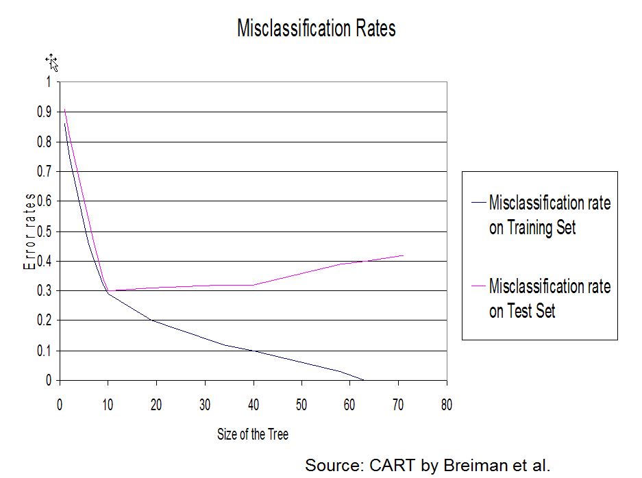
To overcome the overfitting problem (accurate results on the training set but worse results on the test set), a solution is to start from a maximal tree (where all leaves are homogeneous), and use iterative pruning to obtain an optimal subtree for a given quality criterion.
Remark
Remark 4. This step-by-step methodology does not necessarily lead to a global optimal subtree but it is a computationally plausible solution.
2.5.2 A penalized criterion
The idea of pruning is to penalize the risk by the complexity of the model.
A penalized version of the empirical risk that takes into account the complexity of the tree can be defined through:
\[R_\gamma (\mathcal T) = R (\mathcal T) + \gamma | \mathcal T |\] where \(|\mathcal T|\) is the number of leaves of the tree \(\mathcal T\).
2.5.3 Iterative pruning
When \(\gamma=0\), \(R_\gamma (\mathcal T) = R (\mathcal T)\) and hence the subtree of \(\mathcal T\) optimizing this criterion is very often \(\mathcal T\) itself.
When \(\gamma\) increases, one of the nodes’ split, \(\mathcal{S}_{j}\) appears such that: \[R_\gamma (\mathcal T) > R_\gamma (\mathcal{T}^{-\mathcal{S}_{j}})\] where \(\mathcal{T}^{-\mathcal{S}_{j}}\) is the tree where the split \(\mathcal{S}_{j}\) has been removed. Let us call \(\mathcal{T}_{K-1}\) this new tree.
This process is iterated to obtain a sequence of trees \[\mathcal{T} \supset \mathcal{T}_{K-1} \supset \ldots \supset \mathcal{T}_{1}\] where \(\mathcal{T}_{1}\) is the tree restricted to its root.
2.5.4 Choosing the optimal subtree
The optimal subtree is chosen by validation or cross-validation by the following algorithm:
Algorithm for cross validation choice
- Build the maximal tree, \(\mathcal{T}\)
- Build the sequence of subtrees \((\mathcal{T}_k)_{k=1,\ldots,K}\)
- By validation (or cross validation), evaluate the risks \(R_{\operatorname{CV}} (\mathcal{T}_{k})\) for \(1 \leq k \leq K\) (that risk as a function of the number of leaves can be represented graphically).
- Finally, choose \(k\) which minimizes \(R_{\operatorname{CV}} (\mathcal{T}_{k})\)
In R, the rpart function carries out step 3 using a 10 fold cross validation where the data is divided into 10 subsets of equal size (at random) and then the tree is grown leaving out one of the subsets and the performance assessed on the subset that was left out. This is done for each of the 10 sets. The average risk is then assessed.
We can then use the plot of the cross-validated error by the number of leaves to decide on trade-off between the complexity of the model and its accuracy.
The most naive rule for step 4 is to minimize the cross validation relative error.
An alternative that is often preferred is the “1-SE rule” which uses the largest value of the complexity parameter with a risk that is within one standard deviation of the minimum (represented by a dashed line in the rpart::plotcp function).
Remark
Remark. More details can be found on pages 12-14 of the introduction to rpart by Therneau and Atkinson (2023).
References
Breiman, Leo, Jerome H. Friedman, Richard A. Olshen, and Charles J. Stone. 1984. Classification And Regression Trees. 1st ed. Routledge. https://doi.org/10.1201/9781315139470.
Therneau, Terry M, and Elizabeth J Atkinson. 2023. “An Introduction to Recursive Partitioning Using the RPART Routines.” https://cran.r-project.org/web/packages/rpart/vignettes/longintro.pdf.