Case Study in `R`: Old French administrative regions

Last updated on January 5, 2026

1 Nature of the data

The data set

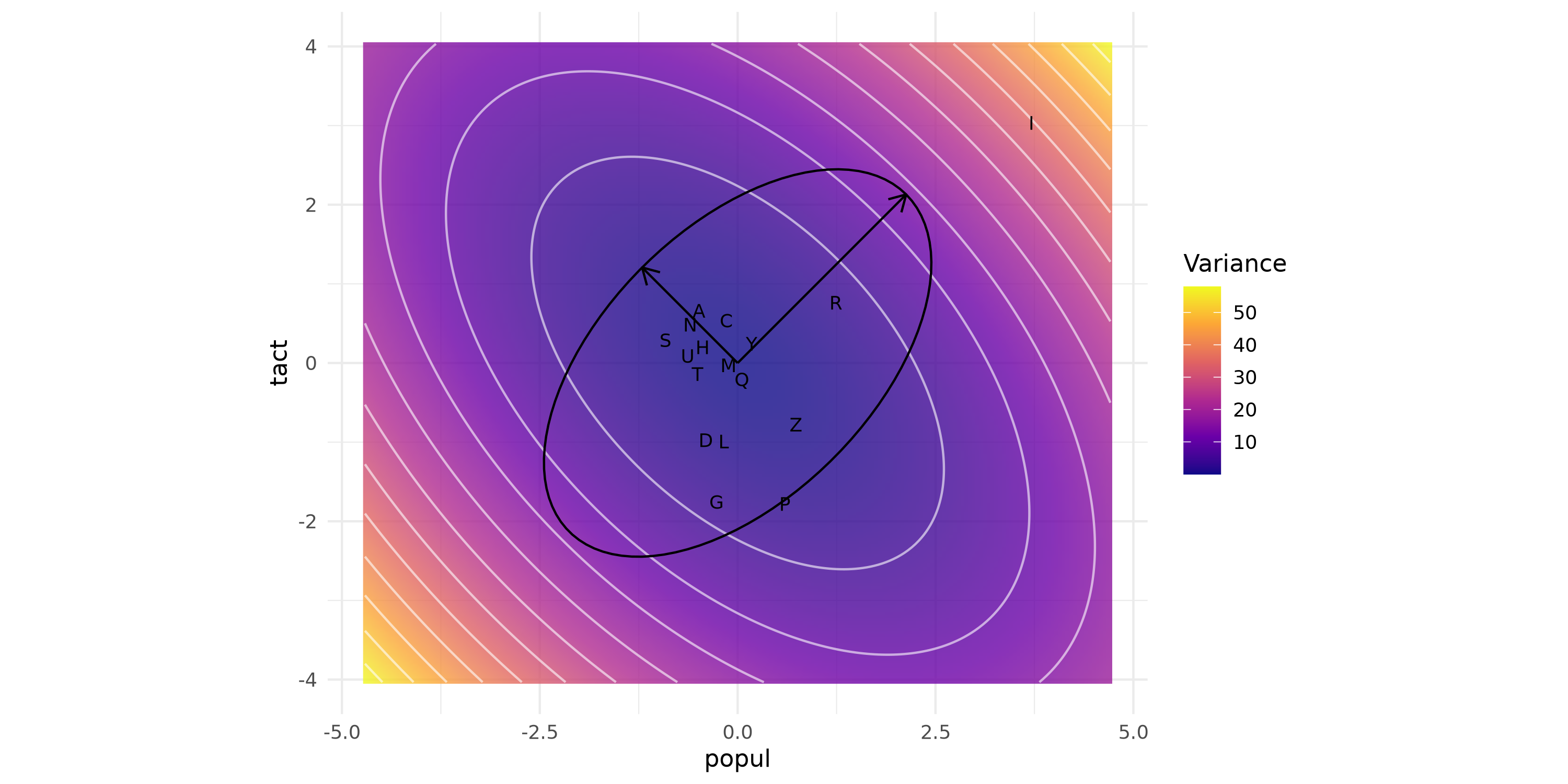
The application example deals with the 21 French regions except Corsica (the individuals or cases) characterized by several indicators (the variables).

The considered variables are the following:

POPUL : population of the region (in thousands of individuals)
TACT : activity rate of the region (in percentage)
SUPERF : surface of the region (in square kilometers )
NBENTR : number of firms of the region
NBBREV : number of patents taken out during the year
CHOM : unemployment rate (in percentage)
TELEPH : number of telephone lines in place in the region (in thousands).

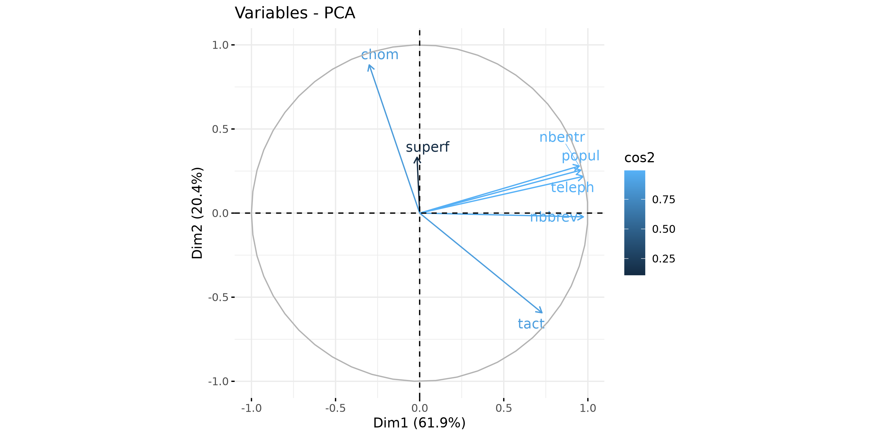
Source: Anne M. Ruiz.

Presentation of the variables

Code

library(FactoMineR)
library(factoextra)
library(ggplot2)
library(corrplot)

X <- read.csv("data/regions.csv", row.names = 1)
X

Table 1: The data table \(\mathbf X\).

	region	popul	tact	superf	nbentr	nbbrev	chom	teleph
A	Alsace	1624	39.14	8280	35976	241	5.2	700
Q	Aquitaine	2795	36.62	41308	85531	256	10.2	1300
U	Auvergne	1320	37.48	26013	40494	129	9.3	600
N	Bas-Norm	1390	38.63	17589	35888	91	9.0	600
O	Bourgogne	1600	38.26	31582	40714	223	8.1	750
B	Bretagne	2795	36.62	27208	73763	296	9.5	1300
C	Centre	2370	38.78	39151	56753	229	7.9	1100
E	Champ-Ard	1340	37.85	25606	24060	155	9.3	550
F	Fr-Comte	1090	37.27	16202	27481	159	7.1	450
H	Hte-Norm	1730	37.80	12317	37461	181	10.8	750
I	Ile-de-Fr	10660	46.04	12012	273604	6722	7.3	5800
G	Lang-Rous	2110	32.12	27376	62202	179	13.2	1000
S	Limousin	720	38.06	16942	21721	73	7.9	350
L	Lorraine	2300	34.34	23547	48353	185	8.6	950
M	Midi-Pyr	2430	37.14	45348	78771	237	9.0	1100
P	Nord-PdC	3960	32.05	12414	78504	278	12.6	1600
Y	Pays-Loir	3060	37.93	32082	72027	339	9.6	1300
D	Picardie	1810	34.39	19399	36285	139	9.8	750
T	Poit-Char	1590	36.82	25809	44598	133	10.1	750
Z	Pr-Cte-Az	4260	34.96	31400	132552	610	11.0	2300
R	Rh-Alpes	5350	39.44	48698	159634	1474	7.4	2500

2 Objectives of PCA

Code

pairs(X[, 2:8])

Figure 1: Scatterplots of initial variables.

3 Principles of PCA

What ‘information’ means

The inertia (total variance) is: 3.5195826^{9}.

3.1 Standardized variables

Why we standardize

Code

vars <- apply(X[, 2:8], 2, var)
df_var <- data.frame(
  Variable = names(vars),
  Variance = vars
)

ggplot(df_var, aes(x = Variable, y = Variance)) +
  geom_col() +
  theme_minimal() +
  labs(y = "Variance", x = "")

Figure 2: Variance of the original variables (before standardization).

Scatterplots matrix of scaled data set

Code

pairs(scale(X[, 2:8]))

Figure 3: Scatterplots of standardized variables.

3.2 Principal components

Heuristics

Code

library(ggplot2)
library(ellipse)
library(viridis)

# Select and scale two variables
vars <- 2:3
X_small <- as.data.frame(scale(X[, vars]))
colnames(X_small) <- c("x", "y")

# Covariance matrix
S <- cov(X_small)

# Determine bounding box
lim <- apply(X_small, 2, function(x) max(abs(x))) + 1
x_seq <- seq(-lim[1], lim[1], length.out = 200)
y_seq <- seq(-lim[2], lim[2], length.out = 200)

# Grid for heatmap
grid <- expand.grid(x = x_seq, y = y_seq)
grid$qform <- rowSums((as.matrix(grid) %*% S) * as.matrix(grid))

# Covariance ellipse (95% confidence)
df_ell <- as.data.frame(ellipse(S, level = 0.95))
colnames(df_ell) <- c("x", "y")

# Eigenvectors scaled to touch ellipse
eig <- eigen(S)
scale_factor <- sqrt(qchisq(0.95, df = 2))
vecs <- data.frame(
  x0 = 0, y0 = 0,
  x1 = scale_factor * sqrt(eig$values) * eig$vectors[1, ],
  y1 = scale_factor * sqrt(eig$values) * eig$vectors[2, ]
)

# Plot
ggplot() +
  geom_raster(data = grid, aes(x, y, fill = qform), interpolate = TRUE, alpha = 0.8) +
  geom_contour(data = grid, aes(x, y, z = qform), color = "white", alpha = 0.6) +
  geom_text(data = X_small, aes(x, y, label = rownames(X_small)), size = 3, check_overlap = TRUE) +
  geom_path(data = df_ell, aes(x, y)) +
  geom_segment(data = vecs, aes(x = x0, y = y0, xend = x1, yend = y1),
               arrow = arrow(length = unit(0.3, "cm"))) +
  coord_fixed(xlim = c(-lim[1], lim[1]), ylim = c(-lim[2], lim[2])) +
  scale_fill_viridis_c(option = "plasma") +
  labs(
    x = colnames(X)[vars[1]],
    y = colnames(X)[vars[2]],
    fill = "Variance",
  ) +
  theme_minimal()

Figure 4: Variance of the projected data as a function of direction.

Definition

Principal components & scores

Code

res_pca <- PCA(X[, 2:8], scale.unit = TRUE, graph = FALSE)
head(res_pca$ind$coord)

       Dim.1      Dim.2       Dim.3      Dim.4       Dim.5
A -0.2809441 -2.7349067 -0.76838621 -0.7398786 -0.21841544
Q -0.1101912  0.9983034  1.19600815  0.1937697 -0.01363514
U -0.9339127 -0.3488172  0.09005665  0.3516347  0.06681602
N -0.7968759 -0.8950699 -0.52292379  0.4893417 -0.18942068
O -0.5900488 -0.7848025  0.74941316  0.1498634  0.12968496
B -0.1258669  0.3093384  0.08262498 -0.0956553 -0.13360686

Principal axes & loadings

Code

res_pca$var$coord

             Dim.1       Dim.2       Dim.3       Dim.4       Dim.5
popul   0.95783293  0.25547751 -0.04443395 -0.08882877 -0.04217485
tact    0.72719947 -0.59263111  0.14930416  0.30773685 -0.05438998
superf -0.01552123  0.33187207  0.94202679  0.03199371  0.03341067
nbentr  0.94885018  0.27975109  0.08090534 -0.07645690 -0.05962944
nbbrev  0.97349367 -0.02238409 -0.15753009  0.06195308  0.15175965
chom   -0.29985584  0.88117115 -0.25791205  0.25882737 -0.01061849
teleph  0.97224065  0.21803299 -0.05362987 -0.04974105 -0.01427041

Connection with Courant–Fisher min-max theorem

Code

res_pca$eig

        eigenvalue percentage of variance cumulative percentage of variance
comp 1 4.329675886            61.85251266                          61.85251
comp 2 1.429382161            20.41974516                          82.27226
comp 3 1.012436783            14.46338261                          96.73564
comp 4 0.182765737             2.61093910                          99.34658
comp 5 0.032756318             0.46794741                          99.81453
comp 6 0.010720602             0.15315145                          99.96768
comp 7 0.002262513             0.03232161                         100.00000

Properties

Code

cov(res_pca$ind$coord)

              Dim.1         Dim.2         Dim.3         Dim.4         Dim.5
Dim.1  4.546160e+00 -3.751882e-17  1.020234e-16  4.651227e-18 -2.808897e-17
Dim.2 -3.751882e-17  1.500851e+00 -2.278722e-17 -2.041722e-16 -1.346139e-17
Dim.3  1.020234e-16 -2.278722e-17  1.063059e+00  1.378943e-16  2.247958e-17
Dim.4  4.651227e-18 -2.041722e-16  1.378943e-16  1.919040e-01 -8.496757e-18
Dim.5 -2.808897e-17 -1.346139e-17  2.247958e-17 -8.496757e-18  3.439413e-02

Geometric approach to PCA

Code

svd(scale(X[, 2:8]))$d

[1] 9.3055638 5.3467414 4.4998595 1.9118877 0.8093988 0.4630465 0.2127211

4 Component selection criteria

Percentage of explained variance criterion

Code

fviz_screeplot(res_pca, addlabels = TRUE)

Kaiser criterion

Code

res_pca$eig[, 1] > 1

comp 1 comp 2 comp 3 comp 4 comp 5 comp 6 comp 7 
  TRUE   TRUE   TRUE  FALSE  FALSE  FALSE  FALSE

Scree test criterion

Code

plot(res_pca$eig[, 1], type = "b", xlab = "Component", ylab = "Eigenvalue")

5 Interpreting PCA

5.1 Interpreting the components

Presentation of the problem

Code

fviz_pca_var(res_pca, col.var = "contrib", repel = TRUE)

Interpretation of the loadings

Code

barplot(res_pca$var$contrib[, 1], las = 2, main = "Contributions to PC1")

Figure 8

Interpretation of the correlations between the components and the initial variables

Code

fviz_pca_var(res_pca, col.var = "cos2", repel = TRUE)

Correlations between variables and components

Code

res_pca$var$cor

             Dim.1       Dim.2       Dim.3       Dim.4       Dim.5
popul   0.95783293  0.25547751 -0.04443395 -0.08882877 -0.04217485
tact    0.72719947 -0.59263111  0.14930416  0.30773685 -0.05438998
superf -0.01552123  0.33187207  0.94202679  0.03199371  0.03341067
nbentr  0.94885018  0.27975109  0.08090534 -0.07645690 -0.05962944
nbbrev  0.97349367 -0.02238409 -0.15753009  0.06195308  0.15175965
chom   -0.29985584  0.88117115 -0.25791205  0.25882737 -0.01061849
teleph  0.97224065  0.21803299 -0.05362987 -0.04974105 -0.01427041

Space of variables

Code

corrplot(cor(X[, 2:8]), method = "ellipse", type = "upper")

The \(L^2\) Hilbert space of random variables

Code

cos(cor(X[, 2:8]))

           popul      tact    superf    nbentr    nbbrev      chom    teleph
popul  0.5403023 0.8709006 0.9997031 0.5561757 0.6047263 0.9973272 0.5454153
tact   0.8709006 0.5403023 0.9982449 0.8699411 0.7593713 0.7657810 0.8497613
superf 0.9997031 0.9982449 0.5403023 0.9888767 0.9865890 0.9980750 0.9999886
nbentr 0.5561757 0.8699411 0.9888767 0.5403023 0.6281623 0.9969557 0.5546043
nbbrev 0.6047263 0.7593713 0.9865890 0.6281623 0.5403023 0.9672645 0.5861916
chom   0.9973272 0.7657810 0.9980750 0.9969557 0.9672645 0.5403023 0.9951694
teleph 0.5454153 0.8497613 0.9999886 0.5546043 0.5861916 0.9951694 0.5403023

5.2 Interpreting the individuals

Graph of the individuals

Code

fviz_pca_ind(res_pca, repel = TRUE)

Projecting shrinkens the distances

Code

dist(scale(X[, 2:8]))[1:10]

 [1] 4.224496 2.782955 2.230527 2.605100 3.153378 3.149473 2.746772 1.446662
 [9] 3.091541 8.969848

Measure of the quality of representation of the individuals

Code

fviz_cos2(res_pca, choice = "ind")

Contributions of individuals for a component

Code

fviz_contrib(res_pca, choice = "ind", axes = 1)

5.3 The biplot

Code

fviz_pca_biplot(res_pca, repel = TRUE)

6 Additional concepts and extensions

6.1 Size factor

Code

res_pca$var$coord[, 1]

      popul        tact      superf      nbentr      nbbrev        chom 
 0.95783293  0.72719947 -0.01552123  0.94885018  0.97349367 -0.29985584 
     teleph 
 0.97224065

6.2 Rotation methods

Code

varimax(res_pca$var$coord[, 1:2])$loadings


Loadings:
       Dim.1  Dim.2 
popul   0.991       
tact    0.564 -0.750
superf         0.326
nbentr  0.988       
nbbrev  0.940 -0.256
chom           0.927
teleph  0.996       

               Dim.1 Dim.2
SS loadings    4.162 1.597
Proportion Var 0.595 0.228
Cumulative Var 0.595 0.823

6.3 Kernel PCA

Inner products and feature maps

Code

tcrossprod(scale(X[, 2:8]))[1:5, 1:5]

           A           Q           U          N         O
A  8.3294051 -3.57839154  0.83427073  2.6237306 1.5189479
Q -3.5783915  2.36017972 -0.06399258 -1.2684086 0.1931491
U  0.8342707 -0.06399258  1.08397643  1.1176521 0.9028860
N  2.6237306 -1.26840858  1.11765206  1.8933083 0.7864583
O  1.5189479  0.19314906  0.90288605  0.7864583 1.4950391

The kernel trick

Code

exp(-as.matrix(dist(scale(X[, 2:8])))^2)

             A            Q            U            N            O            B
A 1.000000e+00 1.775910e-08 4.329709e-04 6.906778e-03 1.128858e-03 4.802477e-05
Q 1.775910e-08 1.000000e+00 2.809563e-02 1.124625e-03 3.115063e-02 1.774225e-01
U 4.329709e-04 2.809563e-02 1.000000e+00 4.761699e-01 4.615137e-01 2.797030e-01
N 6.906778e-03 1.124625e-03 4.761699e-01 1.000000e+00 1.627678e-01 8.259218e-02
O 1.128858e-03 3.115063e-02 4.615137e-01 1.627678e-01 1.000000e+00 1.503922e-01
B 4.802477e-05 1.774225e-01 2.797030e-01 8.259218e-02 1.503922e-01 1.000000e+00
C 4.922140e-05 8.583465e-02 7.301034e-02 1.118464e-02 4.579741e-01 7.674728e-02
E 5.288761e-04 1.335679e-02 9.052487e-01 5.256336e-01 4.283527e-01 1.631389e-01
F 1.233376e-01 4.938788e-05 1.051446e-01 2.584411e-01 8.882734e-02 1.141115e-02
H 7.066047e-05 3.545014e-04 1.123663e-01 2.739202e-01 6.373210e-03 3.909550e-02
I 1.141458e-35 9.854014e-35 1.972249e-38 4.730269e-37 9.657003e-37 1.221263e-32
G 8.568706e-13 1.030491e-03 2.551458e-04 1.144837e-05 3.806006e-06 1.318856e-03
S 4.073905e-02 1.001321e-04 2.269759e-01 5.495607e-01 1.248511e-01 1.468904e-02
L 2.965734e-04 1.266736e-02 1.875401e-01 5.969587e-02 7.837277e-02 2.738079e-01
M 9.397124e-08 5.204832e-01 2.176028e-02 7.368232e-04 8.021477e-02 6.541731e-02
P 2.368122e-11 1.638722e-05 2.062831e-05 7.202699e-06 1.830922e-07 6.366788e-04
Y 1.173978e-05 3.526855e-01 1.903805e-01 4.217554e-02 1.919420e-01 6.653250e-01
D 5.218626e-05 4.032200e-03 1.985586e-01 9.099440e-02 2.253008e-02 1.432493e-01
T 4.086222e-05 5.464168e-02 7.581883e-01 2.682163e-01 1.849613e-01 3.978916e-01
Z 2.133867e-10 4.181670e-02 2.266968e-04 1.663971e-05 6.879567e-05 3.415675e-02
R 1.863814e-11 2.121879e-04 5.632554e-08 2.555374e-09 2.855881e-06 1.478125e-05
             C            E            F            H            I            G
A 4.922140e-05 5.288761e-04 1.233376e-01 7.066047e-05 1.141458e-35 8.568706e-13
Q 8.583465e-02 1.335679e-02 4.938788e-05 3.545014e-04 9.854014e-35 1.030491e-03
U 7.301034e-02 9.052487e-01 1.051446e-01 1.123663e-01 1.972249e-38 2.551458e-04
N 1.118464e-02 5.256336e-01 2.584411e-01 2.739202e-01 4.730269e-37 1.144837e-05
O 4.579741e-01 4.283527e-01 8.882734e-02 6.373210e-03 9.657003e-37 3.806006e-06
B 7.674728e-02 1.631389e-01 1.141115e-02 3.909550e-02 1.221263e-32 1.318856e-03
C 1.000000e+00 5.679885e-02 4.250161e-03 2.112311e-04 3.117545e-34 4.517646e-07
E 5.679885e-02 1.000000e+00 1.139101e-01 1.167847e-01 3.773518e-39 1.135826e-04
F 4.250161e-03 1.139101e-01 1.000000e+00 1.284469e-02 3.928947e-39 1.322653e-07
H 2.112311e-04 1.167847e-01 1.284469e-02 1.000000e+00 2.109986e-37 5.373917e-04
I 3.117545e-34 3.773518e-39 3.928947e-39 2.109986e-37 1.000000e+00 9.757572e-45
G 4.517646e-07 1.135826e-04 1.322653e-07 5.373917e-04 9.757572e-45 1.000000e+00
S 5.201577e-03 2.778943e-01 7.288398e-01 4.693361e-02 3.875915e-40 5.120755e-07
L 1.219225e-02 1.194987e-01 6.577641e-02 1.921486e-02 7.525993e-38 9.310236e-04
M 3.275572e-01 1.139259e-02 1.082854e-04 3.813679e-05 6.661700e-36 2.071673e-05
P 1.165098e-08 8.353473e-06 1.472273e-07 9.464203e-04 9.980663e-38 5.358478e-02
Y 2.167648e-01 1.232343e-01 3.007894e-03 1.199323e-02 1.100141e-31 2.546934e-04
D 1.288193e-03 1.480063e-01 3.328911e-02 1.271691e-01 2.318841e-40 8.535583e-03
T 2.941191e-02 6.180823e-01 2.759729e-02 1.842702e-01 2.647023e-38 3.507403e-03
Z 1.851795e-04 5.973656e-05 3.412430e-07 6.320986e-05 3.835061e-28 1.890485e-03
R 3.213490e-04 1.539799e-08 3.651416e-10 2.940565e-11 5.079321e-21 1.447010e-12
             S            L            M            P            Y            D
A 4.073905e-02 2.965734e-04 9.397124e-08 2.368122e-11 1.173978e-05 5.218626e-05
Q 1.001321e-04 1.266736e-02 5.204832e-01 1.638722e-05 3.526855e-01 4.032200e-03
U 2.269759e-01 1.875401e-01 2.176028e-02 2.062831e-05 1.903805e-01 1.985586e-01
N 5.495607e-01 5.969587e-02 7.368232e-04 7.202699e-06 4.217554e-02 9.099440e-02
O 1.248511e-01 7.837277e-02 8.021477e-02 1.830922e-07 1.919420e-01 2.253008e-02
B 1.468904e-02 2.738079e-01 6.541731e-02 6.366788e-04 6.653250e-01 1.432493e-01
C 5.201577e-03 1.219225e-02 3.275572e-01 1.165098e-08 2.167648e-01 1.288193e-03
E 2.778943e-01 1.194987e-01 1.139259e-02 8.353473e-06 1.232343e-01 1.480063e-01
F 7.288398e-01 6.577641e-02 1.082854e-04 1.472273e-07 3.007894e-03 3.328911e-02
H 4.693361e-02 1.921486e-02 3.813679e-05 9.464203e-04 1.199323e-02 1.271691e-01
I 3.875915e-40 7.525993e-38 6.661700e-36 9.980663e-38 1.100141e-31 2.318841e-40
G 5.120755e-07 9.310236e-04 2.071673e-05 5.358478e-02 2.546934e-04 8.535583e-03
S 1.000000e+00 4.349412e-02 1.612586e-04 2.287488e-07 5.268328e-03 4.335253e-02
L 4.349412e-02 1.000000e+00 7.014004e-03 5.781880e-04 6.234285e-02 5.057860e-01
M 1.612586e-04 7.014004e-03 1.000000e+00 1.146129e-07 1.865512e-01 8.932504e-04
P 2.287488e-07 5.781880e-04 1.146129e-07 1.000000e+00 4.568365e-05 4.583393e-03
Y 5.268328e-03 6.234285e-02 1.865512e-01 4.568365e-05 1.000000e+00 2.480950e-02
D 4.335253e-02 5.057860e-01 8.932504e-04 4.583393e-03 2.480950e-02 1.000000e+00
T 7.069353e-02 2.076496e-01 1.978570e-02 3.333554e-04 2.339776e-01 3.411862e-01
Z 3.735894e-07 1.441739e-03 2.656056e-03 2.902219e-03 2.297907e-02 5.793443e-04
R 1.437626e-10 6.058970e-08 6.152205e-04 5.284868e-13 1.366085e-04 3.957826e-10
             T            Z            R
A 4.086222e-05 2.133867e-10 1.863814e-11
Q 5.464168e-02 4.181670e-02 2.121879e-04
U 7.581883e-01 2.266968e-04 5.632554e-08
N 2.682163e-01 1.663971e-05 2.555374e-09
O 1.849613e-01 6.879567e-05 2.855881e-06
B 3.978916e-01 3.415675e-02 1.478125e-05
C 2.941191e-02 1.851795e-04 3.213490e-04
E 6.180823e-01 5.973656e-05 1.539799e-08
F 2.759729e-02 3.412430e-07 3.651416e-10
H 1.842702e-01 6.320986e-05 2.940565e-11
I 2.647023e-38 3.835061e-28 5.079321e-21
G 3.507403e-03 1.890485e-03 1.447010e-12
S 7.069353e-02 3.735894e-07 1.437626e-10
L 2.076496e-01 1.441739e-03 6.058970e-08
M 1.978570e-02 2.656056e-03 6.152205e-04
P 3.333554e-04 2.902219e-03 5.284868e-13
Y 2.339776e-01 2.297907e-02 1.366085e-04
D 3.411862e-01 5.793443e-04 3.957826e-10
T 1.000000e+00 1.419363e-03 3.879027e-08
Z 1.419363e-03 1.000000e+00 8.524055e-05
R 3.879027e-08 8.524055e-05 1.000000e+00

Kernel PCA

Code

# Illustration only (no computation)

7 Conclusion

Code

fviz_eig(res_pca, addlabels = TRUE)

Case Study in R: Old French administrative regions

1 Nature of the data

The data set

Presentation of the variables

2 Objectives of PCA

3 Principles of PCA

What ‘information’ means

3.1 Standardized variables

Why we standardize

Scatterplots matrix of scaled data set

3.2 Principal components

Heuristics

Definition

Principal components & scores

Principal axes & loadings

Connection with Courant–Fisher min-max theorem

Properties

Geometric approach to PCA

4 Component selection criteria

Percentage of explained variance criterion

Kaiser criterion

Scree test criterion

5 Interpreting PCA

5.1 Interpreting the components

Presentation of the problem

Interpretation of the loadings

Interpretation of the correlations between the components and the initial variables

Correlations between variables and components

Space of variables

The \(L^2\) Hilbert space of random variables

5.2 Interpreting the individuals

Graph of the individuals

Projecting shrinkens the distances

Measure of the quality of representation of the individuals

Contributions of individuals for a component

5.3 The biplot

6 Additional concepts and extensions

6.1 Size factor

6.2 Rotation methods

6.3 Kernel PCA

Inner products and feature maps

The kernel trick

Kernel PCA

7 Conclusion

Case Study in `R`: Old French administrative regions