or quantitative (numerical) \(\rightarrow\)regression trees.
This means that decision tree learning is a supervized method (contrarily to PCA and clustering that are unsupervized methods): part of machine learning algorithms that “learn” from the data.
Predictors are either numerical or categorical.
A decision tree is defined using a training sample and tested on a test sample (split the original sample in two samples).
The method is nonlinear.
Different algorithms exist. We consider only CART developed by Breiman et al. (1984).
1.2 Examples
Predict the land use of a given area (agriculture, forest, etc.) given satellite information, meteorological data, socio-economic information, prices information, etc.
Predict high risk for heart attack:
University of California: a study into patients after admission for a heart attack.
19 variables collected during the first 24 hours for 215 patients (for those who survived the 24 hours)
Question: Can the high risk (will not survive 30 days) patients be identified?
Determine how computer performance is related to a number of variables which describe the features of a PC (the size of the cache, the cycle time of the computer, the memory size and the number of channels. Both the last two were not measured but minimum and maximum values obtained).
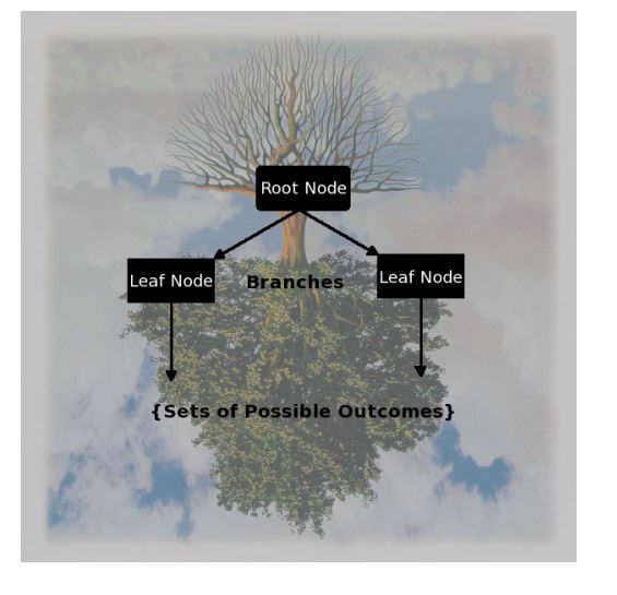
The last level of nodes are the leaf nodes and contain the final classification.
The intermediate nodes are child nodes.
Binary trees (two child nodes) are the most popular type of tree. However, M-ary trees (M branches at each node) are possible.
Nodes contain one question. In a binary tree, by convention if the answer to a question is “yes", the left branch is selected. Note that the same question can appear in multiple places in the tree.
Key questions include how to grow the tree, how to stop growing, and how to prune the tree to increase generalization (good results should not be obtained only on the training set).
1.4 When to use decision trees?
Decision trees are well designed for
problems with a big number of variables (a variable selection is included in the method);
providing an intuitive interpretation with a simple graphic;
solving either regression and classification problems with quantitative or qualitative predictors, hence the name CART.
but they face several difficulties:
they need a large training dataset to be efficient;
as they select the variables hierarchically, they can fail to find a global optimum.
2 Procedure
2.1 Overview
The algorithm is based on two steps:
a recursive binary partitioning of the feature space spanned by the predictor variables into increasingly homogeneous groups with respect to the response variable as measured by:
For regression: Mean squared error.
For classification (with classes \(k=1,2,\dots\)): the Gini index (or entropy or misclassification rate).
a pruning algorithm of the tree when it is too complex.
Figure 3: This tree is too complex, it needs to be pruned!
The subgroups of data created by the partitioning are called nodes.
For regression trees the predicted (fitted) value at a node is just the average value of the response variable for all observations in that node.
For classification trees the predicted value is the class in which there is the largest number of the observations at the node.
For classification trees one also gets the estimated probability of membership in each of the classes from the proportion of the observations at the node in each of the classes.
The subgroups of data created by the partitioning are called nodes.
At each step, an optimization is carried out to select:
A node,
A predictor variable,
A cut-off value if the predictor variable is numerical, or a group of modalities if the predictor variable is categorical,
That maximizes the (percentage) decrease in the objective function (homogeneity measure).
2.2 Notations
The data is built from a pair of random variables, \((X,Y)\), where \(X\) is made of \(p\) qualitative or quantitative predictors, \(X^1, \dots, X^p\), and \(Y\) is a qualitative (classification) or quantitative (regression) variable to predict from \(X\).
The data consists in \(n\) i.i.d. observations \((x_1,y_1), \dots, (x_n,y_n)\) of \((X,Y)\).
As explained previously, building a decision tree aims at finding a series of:
nodes, which are defined by the choice of a variable\(X^k\),
splits deduced from this variable and a threshold\(\tau\), dividing the training sample into two subsamples: \(\{i:\ x_i^k < \tau\}\) and \(\{i:\ x_i^k > \tau\}\) (or in two groups of modalities of \(x\) is categorical).
In the following, we will note the nodes with the following convention:
the root will be denoted by \(\mathcal{N}^0\);
the child nodes of the root will be denoted by \(\mathcal{N}^1_k\) with \(k=1,2\);
the child nodes of \(\mathcal{N}^1_k\) will be denoted by \(\mathcal{N}^2_{2k-1+j}\) with \(k=1,2\) and \(j=0,1\) (hence these nodes are indexed from 1 to 4);
…
the nodes at step \(m\) will be denoted by \(\mathcal{N}^m_k\) for \(k=1,\ldots,2^m\) (where, eventually, some of the indexes can be unused): \(\mathcal{N}^m_1\) and \(\mathcal{N}^m_2\) are the child nodes of \(\mathcal{N}^{m-1}_1\), \(\mathcal{N}^m_3\) and \(\mathcal{N}^m_4\) are the child nodes of \(\mathcal{N}^{m-1}_2\), …
…
2.3 Growing the tree
The need of an homogeneity criterion
When splitting \((y_i)_i\) into two groups, we aim at having two non empty groups with \(Y\) values as homogeneous as possible.
Then, we have to define an homogeneity criterion for each node, i.e. a function \[H:\mathcal{N} \rightarrow \mathbb{R}_+\] that is
null if and only if all the individuals that belong to the node have the same \(Y\) value;
large when all the \(Y\) values are very different.
The split of a node \(\mathcal{N}^m_k\) is chosen, among all possible splits, by minimizing the sum of the homogeneity of the corresponding child nodes: \[\arg\max_{\textrm{splits of }\mathcal{N}^m_k} H(\mathcal{N}^m_k) - \left(n_1 H(\mathcal{N}^{m+1}_{2k-1}) + n_2 H(\mathcal{N}^{m+1}_{2k}\right)/(n_1+n_2).\]
Homogeneity of a split
Consider a given node \(\mathcal{N}^m_k\) that has to be split into two classes (two new child nodes) and denote by
\(\textcolor{blue}{n_1}=\sum_{i=1}^n \mathbb{1}_{\left\{y_i \in \mathcal{N}^{m+1}_{2k-1}\right\}}\) and \(\textcolor{blue}{n_2}=\sum_{i=1}^n \mathbb{1}_{\left\{y_i \in \mathcal{N}^{m+1}_{2k}\right\}}\);
for \(j\in\{-1,0\}\) and a regression tree \(\textcolor{blue}{H(\mathcal{N}^{m+1}_{2k+j})}=\sum_{i=1}^n (y_i - \mathcal{Y}_{2k+j})^2\mathbb{1}_{\left\{y_i \in \mathcal{N}^{m+1}_{2k+j}\right\}}\) where \(\mathcal{Y}_{2k+j}\) is the predicted value in node \(\mathcal{N}^{m+1}_{2k+j}\): \(\mathcal{Y}_{2k+j}=\sum_{i=1}^n y_i \mathbb{1}_{\left\{y_i \in \mathcal{N}^{m+1}_{2k+j}\right\}}.\) The sum of squared criterion is replaced by the Gini index for classification trees.
Building a split: small classification example detailed
Code
library(ggplot2)set.seed(0)a <-data.frame(X_1 =rnorm(800), X_2 =rnorm(800), Y =as.factor("A"))b <-data.frame(X_1 =rnorm(200, 2), X_2 =rnorm(200, 2), Y =as.factor("B"))ab <-rbind(a, b)ggplot(ab, aes(X_1, X_2, color = Y, label = Y)) +geom_point()
Figure 4: A two-classes variable to predict with two quantitative predictors \(X_1\) and \(X_2\).
Code
library(parttree)ab_fit <-rpart(Y ~ ., data = ab, minbucket =nrow(ab), cp =0)rpart.plot(ab_fit, box.palette ="RdBu")ggplot(ab, aes(X_1, X_2, color = Y, label = Y)) +geom_point()for (i in1:3) { ab_fit <-rpart(Y ~ ., data = ab, maxdepth = i, cp =-Inf)rpart.plot(ab_fit, box.palette ="RdBu") p <-ggplot(ab, aes(X_1, X_2, color = Y, fill = Y)) +geom_parttree(data = ab_fit, alpha =0.1, flip = i ==1) +geom_point()print(p)}
(a) Depth 1: a root node.
(b) Depth 1: the feature space.
(c) Depth 2: the first split.
(d) Depth 2: partitioning the feature space.
(e) Depth 3: a taller binary tree.
(f) Depth 3: partitioning the feature space again.
(g) Depth 4: an even taller binary tree.
(h) Depth 4: partitioning the feature space even further.
Figure 5: Building splits recursively.
In order to split a node, we need to choose a criterion of inhomogeneity or measure of impurity.
The measure should be at a maximum when a node is equally divided amongst the two classes.
The impurity should be zero if the node is all one class.
The Gini index is the most widely used measure of impurity (at least by CART): \[1 - p_A^2 -p_B^2\] where \(p_A\) and \(p_B\) are respectively the proportion of observations in class A and in class B for a given node
we compute the decrease of the Gini index when splitting a given node in two child nodes by calculating the Gini index at the given node and substract one half of the sum of the Gini indices at the child nodes as illustrated in the small example below.
We select the split (a variable and a threshold) that most decreases the Gini Index. This is done over all possible places for a split and all possible variables to split.
There are two possible variables to split on and each of those can split for a range of values of \(\tau\) i.e.: \(x < \tau\) or \(y < \tau\).
We keep splitting until the terminal nodes have very few cases or are all pure. Note that this seems an unsatisfactory answer to when to stop growing a tree, but it was realized that the best approach is to grow a larger tree than required and then to prune it.
The growing of the tree is stopped if the obtained node is homogeneous or if the number of observations in the nodes is smaller than a fixed number (generally chosen between 1 and 5).
2.5 Pruning the tree
Why and how pruning?
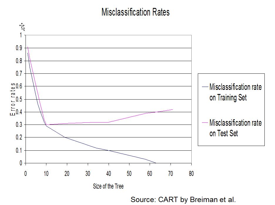
As said earlier it has been found that the best method of arriving at a suitable size for the tree is to grow an overly complex one then to prune it back. The pruning is based on the misclassification rate (number of observations misclassified divided by the total number of observations, see also confusion table). However the error rate will always drop (or at least not increase) with every split. This does not mean however that the error rate on the test data will improve.
Why pruning?
To overcome the overfitting problem (good results on the training set but bad results on the test set).
A solution is to choose one of the subtree of the maximal tree obtained by iterative pruning and to choose the optimal subtree for a given quality criterion. This step-by-step methodology do not necessarily lead to a global optimal subtree but it is a computationally plausible solution.
A penalized criterion
The idea of pruning is to estimate an error criterion penalized by the complexity of the model.
More precisely, suppose that we have obtained the tree \(\mathcal{T}\) with leafs \(\mathcal{F}_1\), …, \(\mathcal{F}_K\) (so \(K\) is the number of leafs) having predicting values \(\mathcal{Y}_1\), …, \(\mathcal{Y}_K\). Then, the error of \(\mathcal{T}\) is \[\textcolor{blue}{L\mathcal{T}}=\sum_{k=1}^K L\mathcal{F}_k\qquad \mbox{ where }\textcolor{blue}{L\mathcal{F}_k} = \sum_{i:\ x_i\in\mathcal{F}_k} (y_i-\mathcal{Y}_k)^2\] for the regression case and the misclassification rate for the classification case.
Hence, a penalized version of the error that takes into account the complexity of the tree can be defined through: \[\textcolor{blue}{L_\gamma\mathcal{T}} = L\mathcal{T} + \gamma K.\] where \(K\) is the size of the tree (number of terminal nodes).
Iterative pruning
When \(\gamma=0\), \(L_\gamma\mathcal{T}=L\mathcal{T}\) and hence the tree optimizing this criterion is \(\mathcal{T}\) (which has been designed for).
When \(\gamma\) is increasing, one of the nodes’ split, \(\mathcal{S}_{j}\) appears such that: \[L_\gamma \mathcal{T} > L_\gamma \mathcal{T}^{-\mathcal{S}_{j}}\] where \(\mathcal{T}^{-\mathcal{S}_{j}}\) is the tree where the split \(\mathcal{S}_{j}\) has been removed. Let us call \(\mathcal{T}_{K-1}\) this new tree.
This process is iterated to obtain a sequence of trees \[\mathcal{T} \supset \mathcal{T}_{K-1} \supset \ldots \mathcal{T}_{1}\] where \(\mathcal{T}_{1}\) is the tree restricted to its root.
Choosing the optimal subtree
The optimal subtree is chosen by validation or cross-validation by the following algorithm: Algorithm for cross validation choice
Build the maximal tree, \(\mathcal{T}\)
Build the sequence of subtrees \((\mathcal{T}_k)_{k=1,\ldots,K}\)
By validation (or cross validation), evaluate the errors\(L\mathcal{T}_{k}\) for \(k=1,\ldots,K\)
Build the graphic of \(L\mathcal{T}_{k}\) in function of \(k=1,\ldots,K\)
Finally, choose \(k\) which minimizes \(L\mathcal{T}_{k}\)
Pruning a tree with the rpart R function
One version of the method carries out a 10 fold cross validation where the data is divided into 10 subsets of equal size (at random) and then the tree is grown leaving out one of the subsets and the performance assessed on the subset left out from growing the tree. This is done for each of the 10 sets. The average performance is then assessed.
This is all done by the command rpart in R and the results are accessible using printcp and plotcp where cp denotes the complexity parameter (\(\gamma\) for printcp but geometric mean of the interval bounds for plotcp).
We can then use this information to decide how complex (determined by the size of cp) the tree needs to be.
The possible rules are to minimize the cross validation relative error (xerror), or to use the “1-SE rule” which uses the largest value of cp with the “xerror” within one standard deviation of the minimum. This rule is often preferred (see the dashed line in the “plotcp” function).
More details can be found on pages 12, 13 and 14 of Therneau and Atkinson (2023).
# Datacandidates <-read.table("data_dt.txt", header =TRUE)# Transformation of the variable to predict into a factorcandidates$Res <-as.factor(candidates$Res)candidates
Table 1: Data set on candidates for a job.
Obs
Id
Dip
Test
Exp
Res
1
A
1
5
4
0
2
B
2
3
3
0
3
C
1
4
5
1
4
D
2
3
4
0
5
E
1
4
4
0
6
F
4
3
4
1
7
G
3
4
4
1
8
H
1
1
5
0
9
I
3
2
5
1
10
J
5
4
4
1
# Classification treelibrary(rpart)library(rpart.plot)# Building the tree (prune is not useful here)candidates_fit <-rpart(Res ~ Dip + Test + Exp,data = candidates, method ="class",parms =list(split ="gini"), control =rpart.control(minsplit =2))
# Plotrpart.plot(candidates_fit)
summary(candidates_fit)
Call:
rpart(formula = Res ~ Dip + Test + Exp, data = candidates, method = "class",
    parms = list(split = "gini"), control = rpart.control(minsplit = 2))
  n= 10

    CP nsplit rel error xerror      xstd
1 0.80      0       1.0    2.0 0.0000000
2 0.10      1       0.2    0.2 0.1897367
3 0.01      3       0.0    0.6 0.2898275

Variable importance
 Dip Test  Exp
  67   20   13

Node number 1: 10 observations,    complexity param=0.8
  predicted class=0  expected loss=0.5  P(node) =1
    class counts:     5     5
   probabilities: 0.500 0.500
  left son=2 (6 obs) right son=3 (4 obs)
  Primary splits:
      Dip  < 2.5 to the left,  improve=3.3333330, (0 missing)
      Test < 1.5 to the left,  improve=0.5555556, (0 missing)
      Exp  < 3.5 to the left,  improve=0.5555556, (0 missing)

Node number 2: 6 observations,    complexity param=0.1
  predicted class=0  expected loss=0.1666667  P(node) =0.6
    class counts:     5     1
   probabilities: 0.833 0.167
  left son=4 (4 obs) right son=5 (2 obs)
  Primary splits:
      Exp  < 4.5 to the left,  improve=0.6666667, (0 missing)
      Test < 3.5 to the left,  improve=0.3333333, (0 missing)
      Dip  < 1.5 to the right, improve=0.1666667, (0 missing)

Node number 3: 4 observations
  predicted class=1  expected loss=0  P(node) =0.4
    class counts:     0     4
   probabilities: 0.000 1.000

Node number 4: 4 observations
  predicted class=0  expected loss=0  P(node) =0.4
    class counts:     4     0
   probabilities: 1.000 0.000

Node number 5: 2 observations,    complexity param=0.1
  predicted class=0  expected loss=0.5  P(node) =0.2
    class counts:     1     1
   probabilities: 0.500 0.500
  left son=10 (1 obs) right son=11 (1 obs)
  Primary splits:
      Test < 2.5 to the left,  improve=1, (0 missing)

Node number 10: 1 observations
  predicted class=0  expected loss=0  P(node) =0.1
    class counts:     1     0
   probabilities: 1.000 0.000

Node number 11: 1 observations
  predicted class=1  expected loss=0  P(node) =0.1
    class counts:     0     1
   probabilities: 0.000 1.000
rpart.plot(candidates_fit, extra =101)
rpart.plot(candidates_fit, extra =103)
# Rulesrpart.rules(candidates_fit)
Res
4
0.00
when
Dip
<
3
&
Exp
<
5
10
0.00
when
Dip
<
3
&
Exp
>=
5
&
Test
<
3
11
1.00
when
Dip
<
3
&
Exp
>=
5
&
Test
>=
3
3
1.00
when
Dip
>=
3
# Predictionpredict(candidates_fit, candidates, type ="class")
Breiman, Leo, Jerome H. Friedman, Richard A. Olshen, and Charles J. Stone. 1984. Classification AndRegressionTrees. 1st ed. Routledge. https://doi.org/10.1201/9781315139470.